
Cartographers like to point out that map projections — the mathematical equations that transform latitude and longitude into planar coordinates — cause geometric distortions to occur. However, the magnitude and spatial distribution of these distortions can be complicated to predict, leaving the map user or map-maker in the predicament of not knowing what map projection is best in a particular situation.
Tissot’s Indicatrix
One tool that can be of assistance is Tissot’s Indicatrix. The Indicatrix is named after French cartographer Nicolas Auguste Tissot, who developed the idea in the nineteenth century. The math behind the Indicatrix is (obviously) complicated, but the concept is straightforward. Imagine drawing a series of circles, each with the same radius, on the globe at the intersection of lines of latitude and longitude (Fig. 1).
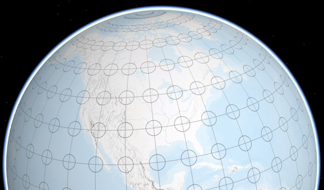
Figure 1. Indicatrix circles on the globe
If we assume a spherical model of the earth, each of these circles will have the same area, since each has the same radius. When we use a particular map projection to make a map, linear distortion is introduced. The pattern of linear distortion tells us whether we have a conformal projection (one which preserves shape), an equal area projection (one which preserves area), or a projection that is neither conformal nor equal area.
If the linear distortion is the same in all directions for any given point on the map, the circles on the globe will still be circles on the map. Thus, at any given point, shape is preserved, and so we classify the projection as conformal, or shape-preserving. But, while linear distortion is the same at ANY point, it is not the same at EVERY point. In other words, some circles on the map are larger than others. This means the projection is not equal area, since the amount of areal distortion varies over the map.
Figure 2 illustrates this situation for the famous Mercator projection. On this projection, the circles get larger as we move away from the equator, indicating larger areal distortion toward the poles. However, since the circles on the globe are still circles on the projection, we know that the Mercator projection preserves shapes locally, and thus is conformal.
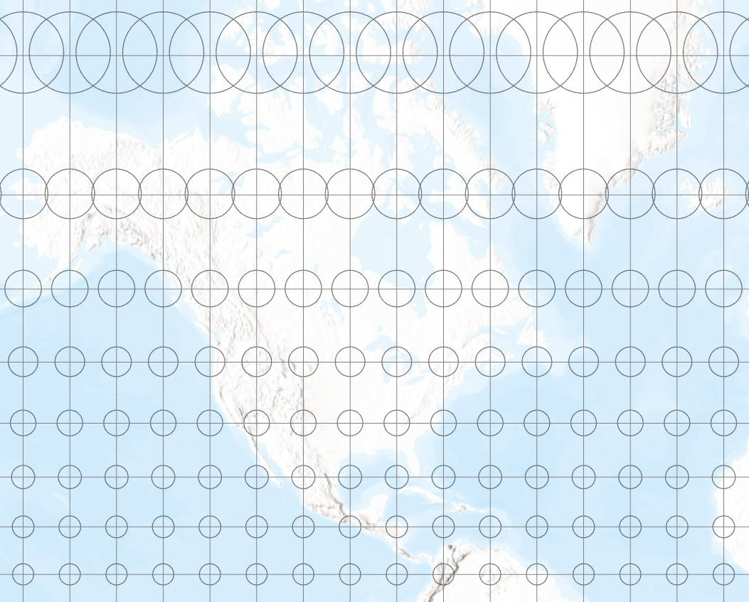
Figure 2 – Indicatrix on the Mercator projection, western half of the northern hemisphere
For some other projections, linear distortion varies in different directions at any point, which means that the circles on the globe are transformed into ellipses. Shape is therefore not preserved, and the projection is not conformal. However, if every ellipse has the same area – the area of an ellipse being the product of pi, the semi-major axis and the semi-minor axis – then the projection is equal area. Figure 3 shows an example for the Lambert Cylindrical Equal Area projection. Notice the great shape distortion as we approach the poles, which is required to maintain the equal area property.
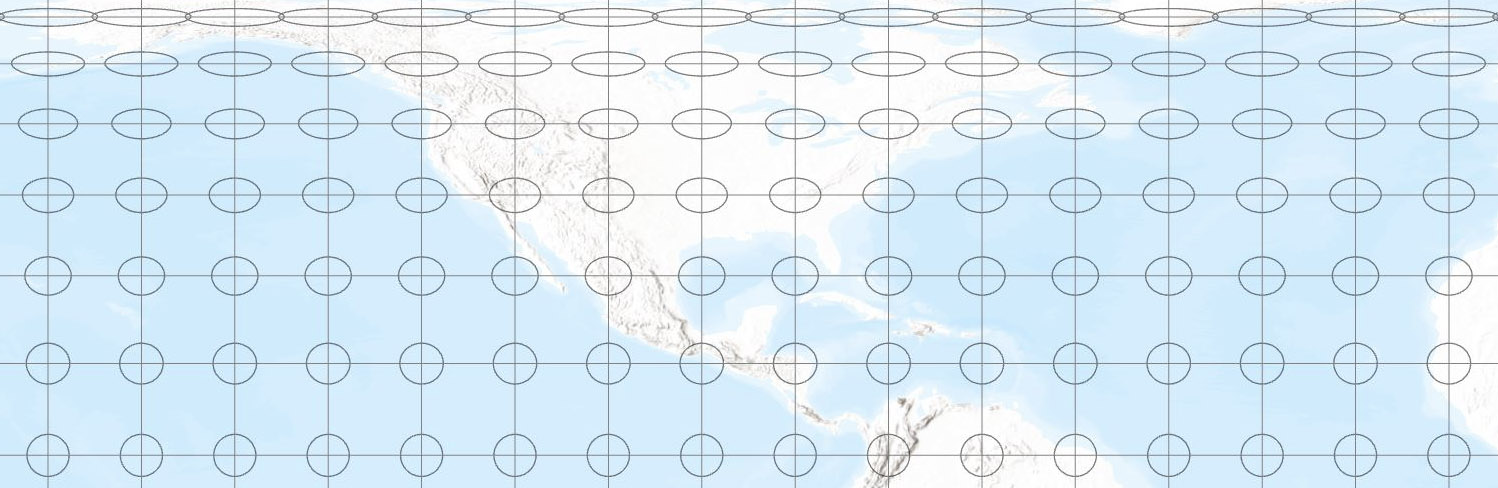
Figure 3 – Indicatrix on the Lambert Cylindrical Equal Area projection, western half of the northern hemisphere
We can have projections that are conformal, or equal area, or neither, but not both. The Gall (or Gall Stereographic) projection is an example of a projection that is neither conformal nor equal area. Not only are the circles on the globe transformed into ellipses, but the ellipses do not all have the same area, getting larger as we move away from the equator. See Figure 4.
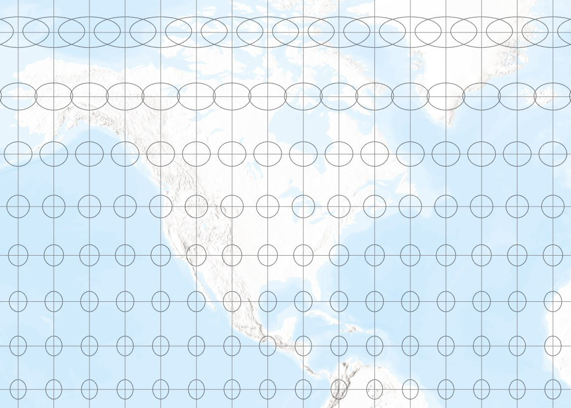
Figure 4 – Indicatrix on the Gall projection, western half of the northern hemisphere
Areal Distortion
It’s fairly easy to create Tissot’s Indicatrix in ArcGIS Pro for any supported projection. Here’s a tutorial on the subject. Below, I will go through an example for the Wisconsin Transverse Mercator projection, also known as WTM. WTM is a special case of a Universal Transverse Mercator (UTM) zone, centered on Wisconsin. Since UTM, and hence WTM, is based on the Mercator projection, we know it is conformal, so we will only need to consider areal distortion. Also, since WTM is based on Mercator, and since most cartographers have been trained to fear this projection, we might be worried that the areal distortion is going to be quite large. Is this the case?
The first step to create the Indicatrix is to use the Create Fishnet tool (Fig. 5). This tool creates a regular grid of points that will serve as the “seeds” for our Indicatrix circles. The parameters for this tool are not very intuitive, so you might let them default the first time you try this, then tweak the parameters to meet your exact needs. For the WTM example, I create a fishnet that covers the state of Wisconsin at a grid size of 40 km. Make sure Create Label Points option is checked. This will produce two new layers – a fishnet line layer and label layer.
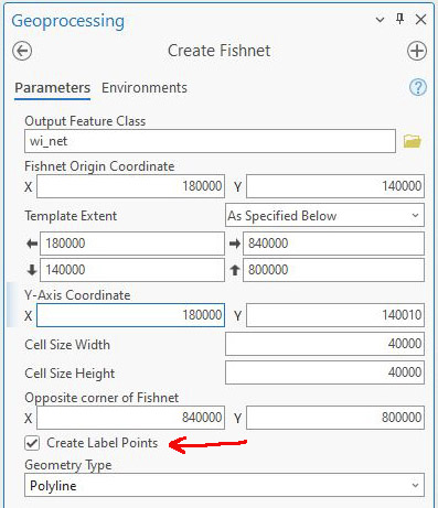
Figure 5 – Create Fishnet tool
Also, make sure the Output Coordinate System in the Environments tab is in agreement with the values you specified (e.g., degrees vs feet or meters). See Figure 6. In this example, I’m using WTM.
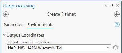
Figure 6 – Environments tab in Create Fishnet tool
The next step is to buffer the fishnet label points layer using the Buffer tool (Fig. 7).
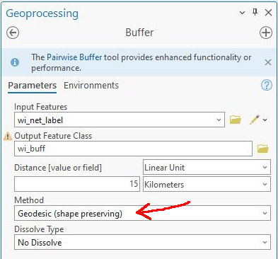
Figure 7 – Using the Buffer tool to make the Indicatrix circles
I’m using a distance of 15 km so that the circles don’t overlap, but are still large enough to see clearly. It is critical that you use the Geodesic option under Method, as this will ensure the circles are the same diameter on the globe.
Next, add three attributes (all doubles) to the buffer attribute table. Two of these attributes will hold the area of the Indicatrix circles on the globe and on the projected WTM map. The third attribute will hold the computed areal distortion values (Fig. 8).
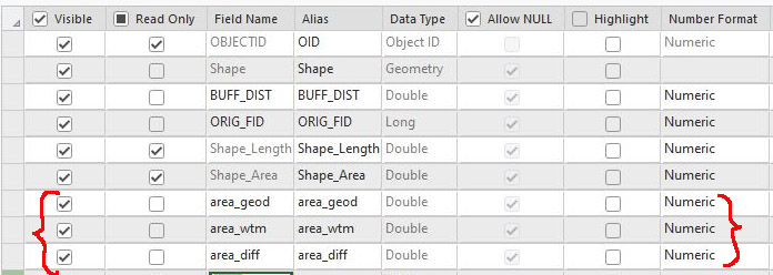
Figure 8 – Adding attributes to the buffer attribute table
Next, compute the area of the Indicatrix circles. To do this, use the Compute Geometry Tool (Fig. 9). Select the “Area (geodesic)” property for the attribute representing the area of the Indicatrix circles on the globe, and select the “Area” property for the attribute representing the area of the Indicatrix circles on the projected map. In this example, the Coordinate System is WTM.
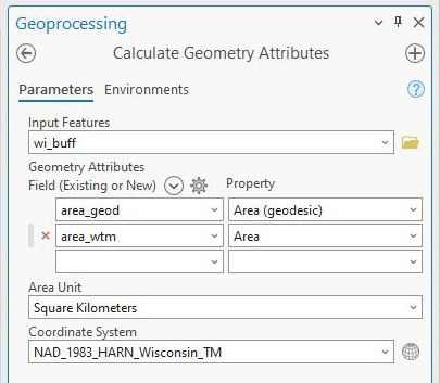
Figure 9 – Computing areas using Calculate Geometry
Next, compute the distortion between the two area attributes you have just calculated. Use the Calculate Field tool, and define the new attribute as the projected area divided by the area on the globe. See Figure 10.
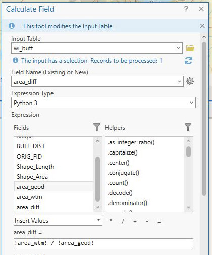
Figure 10 – Calculating areal distortion
That’s it! The areal distortion values you have just computed show whether areas on the WTM projection are smaller than they should be, or larger than they should be.
As you can see from Figure 11, the area of the circles on the globe (area_geod) are the same (except for slight rounding errors) while the area of the circles on the projection (area_wtm) vary from record to record. The distortion (area_diff) can be less than 1 (which means that the area on the projected map is less than it is on the globe) or greater than 1 (which means the opposite).
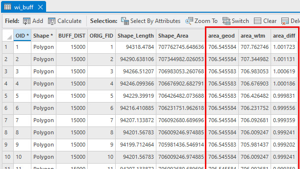
Figure 11 – Results of the calculations
You can visualize the results in a map like the one shown in Figure 12.
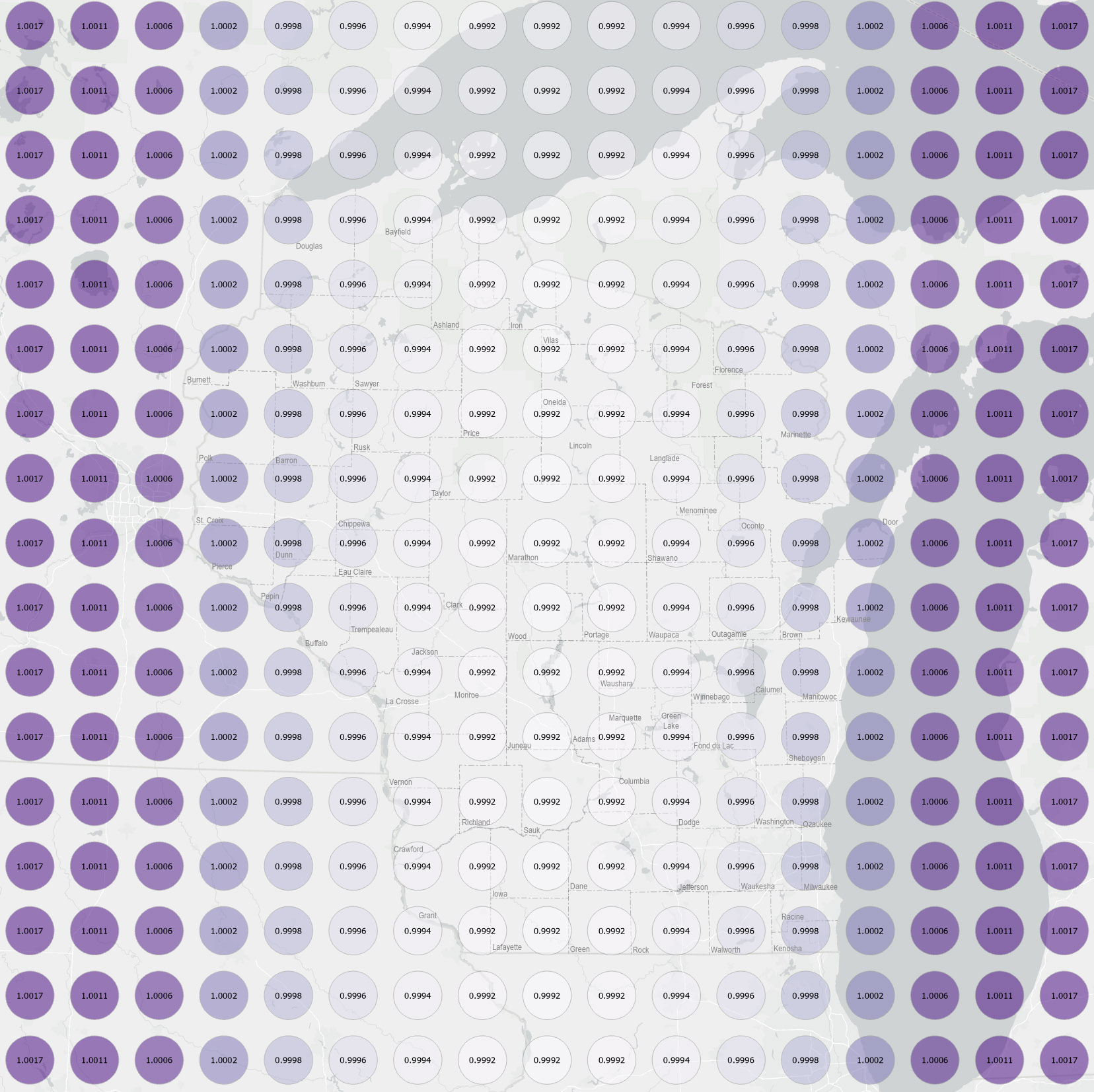
Figure 12 – Areal distortion for Wisconsin for the WTM projection
As you can see, distortion runs in north-south bands, parallel to the central meridian at 90 deg W.
Since the WTM projection uses a scale factor of 0.9996 along the central meridian, the distortion is less than 1 in the center of the map, and greater than 1 at the edges of the map.
Also note that distortion is generally very low (despite the use of a Mercator projection), with the maximum distortion being only a bit more than one part per thousand at the outer edges of the map (i.e., beyond the borders of Wisconsin, where the WTM projection would normally not even be used).
If you want to see some of the mathematics behind these calculations, here’s a good Slack Exchange posting showing how to compute distortion at a point based on the distance between the point and the central meridian, which depends on latitude.
What’s Next?
You can generate your own map for any projection supported in ArcGIS Pro. Doing so will allow you to see how much distortion you have and where it is located. This can be helpful in selecting an appropriate projection for your project, as well as understanding how your analysis might be affected by error.
This blog posting has only covered areal distortion. Shape distortion can also be calculated from Tissot’s Indicatrix, but that will have to be the subject of another posting.